Most AI networking material starts with the switch. This series starts with the GPU, because nothing about an AI fabric makes sense until you’ve seen what a training job actually asks of it: a few huge flows, all starting at the same instant, with every GPU in the job waiting for the slowest one. Get that picture right and PFC thresholds, rails, adaptive routing and SHARP stop being a list of features and become answers to specific problems.
This is the first article in a study series for the NVIDIA Certified Professional AI Networking exam (NCP-AIN). It follows NVIDIA’s public blueprint, explains the reasoning, and sticks to what NVIDIA’s documentation and the published research say. Nothing here comes from the exam itself, and I’m not affiliated with NVIDIA.
In short
- A training step is compute, then a synchronized exchange. The network only matters during the exchange, and then it matters completely: every GPU waits for the slowest transfer.
- Collectives have a cost you can calculate. Ring all-reduce moves about 2S bytes per GPU and pays 2(N − 1) latency steps; trees cut the latency to logarithmic; SHARP and NVLink SHARP cut the bytes.
- Enterprise Clos assumptions break. Few flows defeat ECMP hashing, synchronized fan-in fills buffers in microseconds, and oversubscription stretches every step.
- Stragglers are a network problem with a GPU price. At 1,024 ranks, a 0.1% per-rank hiccup delays 64% of steps; over a month that’s thousands of GPU-hours.
Where this sits in the exam
NVIDIA’s NCP-AIN page lists 70 to 75 questions in 2 hours, no formal prerequisites, and a two-year validity. As of late October 2026 the same page says lab exercises are being added on November 1, with the price rising from $400 to $500. The blueprint weights:
| Domain | Weight | This series |
|---|---|---|
| AI Data Center Design and Optimization | 5% | Articles 1 and 2 |
| NVIDIA Spectrum Networking | 30% | Articles 3 to 7 |
| NVIDIA InfiniBand Networking | 30% | Articles 8 to 12 |
| Kubernetes Integration | 5% | Article 13 |
| Troubleshooting Tools | 20% | Articles 14 to 16 |
| Automation and Configuration | 10% | Articles 17 and 18 |
Design is the smallest domain by weight, and the one every other domain leans on. When the troubleshooting domain asks why a job is slow, or the Spectrum domain asks why RoCE needs ECN marking, the answer usually starts here.
One training step, from the network’s point of view
Photo: 极客湾 Geekerwan, via Wikimedia Commons, CC BY 3.0; resized.
Data-parallel training repeats one loop millions of times. Every GPU holds a copy of the model (or a shard of it) and its own slice of the batch:
- Forward pass. Each GPU runs its batch through the layers. Pure computation, unless tensor parallelism splits layers across GPUs.
- Backward pass. Gradients are computed layer by layer, last layer first.
- Gradient synchronization. All GPUs combine their gradients so every copy of the model takes the same update: an all-reduce.
- Optimizer step. Each GPU applies the averaged gradients. Then the next step starts.
Frameworks don’t wait for the whole backward pass before talking. PyTorch’s DistributedDataParallel groups gradients into buckets (25 MB by default) and starts all-reducing a bucket as soon as backward has filled it, so most of the communication hides behind computation. Most, not all:
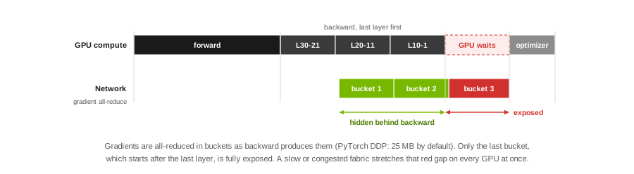
The last bucket can only start once backward has finished, so its transfer time is pure waiting for every GPU in the job. That red gap is the exposed communication. A slow link, a congested queue or a retransmission stretches it on every GPU at once, every step.
Key point. The network’s job isn’t average throughput. It’s to finish the exposed part of each collective as fast as possible, on every GPU, every step.
Parallelism decides the traffic
Large models combine several kinds of parallelism, and each produces a different pattern with a different home in the network:
| Parallelism | What is split | Communication | Typical size and timing | Where it should run |
|---|---|---|---|---|
| Data (DDP) | The batch | All-reduce of gradients | Model-sized, once per step, overlapped with backward | Scale-out fabric |
| Sharded data (FSDP, ZeRO-3) | Batch, plus parameters, gradients and optimizer state | All-gather of parameters, reduce-scatter of gradients | 1.5× plain data parallelism’s volume (ZeRO paper) | Scale-out fabric |
| Tensor (Megatron-style) | Each layer’s matrices | All-reduce inside every layer: two in forward and two in backward per transformer layer | Small, very frequent, latency-critical | Inside the NVLink domain |
| Pipeline | Groups of layers | Point-to-point send and receive between stages | Activation-sized, steady | Scale-out, between neighbors |
| Expert (mixture of experts) | Experts across GPUs | All-to-all: dispatch tokens to experts, combine results | Bursty, every MoE layer | NVLink domain if it fits, else scale-out |
The column on the right is the design. Tensor parallelism generates the chattiest, most latency-sensitive traffic, so it belongs inside the NVLink domain, which is why NVIDIA builds eight-GPU servers and 72-GPU racks around it. What crosses the scale-out fabric is mostly data-parallel and pipeline traffic: large, periodic, and synchronized across thousands of GPUs. That’s the traffic the rest of this series designs for.
The collectives, with the math
NCCL, NVIDIA’s collective communications library, implements every operation above over NVLink, PCIe, InfiniBand and RoCE, and picks an algorithm for each call. Four operations cover almost everything a fabric sees. For N GPUs, S the buffer size in bytes, B the per-GPU link bandwidth and α the latency of one step:
| Operation | Result | Bytes each GPU sends (ring) | Time model (ring) |
|---|---|---|---|
| Reduce-scatter | Each GPU gets one summed 1/N of the buffer | (N − 1)/N × S | (N − 1)α + (N − 1)/N × S/B |
| All-gather | Each GPU gets everyone’s chunk | (N − 1)/N × S | (N − 1)α + (N − 1)/N × S/B |
| All-reduce | Every GPU gets the full sum | 2(N − 1)/N × S | 2(N − 1)α + 2(N − 1)/N × S/B |
| All-to-all | Each GPU sends a distinct 1/N to every other | (N − 1)/N × S | Bounded by the fabric’s bisection bandwidth |
| Broadcast | One GPU’s buffer reaches all | S (pipelined) | About S/B for large buffers |
Ring all-reduce
A ring all-reduce is a reduce-scatter followed by an all-gather. The GPUs form a logical ring, the buffer is cut into N chunks, and in each of N − 1 steps every GPU sends one chunk to its neighbor and adds what it receives. Then N − 1 more steps circulate the finished sums.
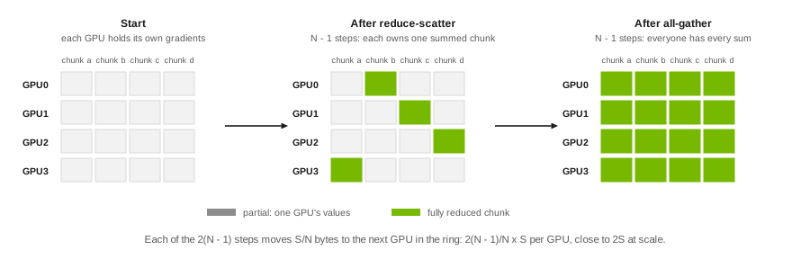
The bandwidth term is excellent: each GPU sends about 2S no matter how many GPUs there are, and every link is busy in every step. The latency term is the problem: 2(N − 1) steps, each paying α. With an illustrative α of 10 µs and 400 Gb/s per GPU (B = 50 GB/s):
| Buffer S | GPUs N | Bandwidth term | Latency term 2(N − 1)α | Dominated by |
|---|---|---|---|---|
| 25 MB (one DDP bucket) | 64 | 0.98 ms | 1.26 ms | Both |
| 25 MB | 1,024 | 1.00 ms | 20.5 ms | Latency |
| 2 GB | 1,024 | 80 ms | 20.5 ms | Bandwidth |
At scale, a flat ring spends more time paying per-step latency than moving bytes for anything but the largest buffers. NCCL answers this in three ways.
Trees, and why NCCL has both
NCCL 2.4 added double binary trees: two complementary binary trees, each carrying half the data, so every GPU is an interior node in at most one. NVIDIA describes the result as full bandwidth with logarithmic latency. With the same α at 1,024 GPUs, the latency term drops from 2 × 1,023 steps to about 2 × log₂(1,024) = 20 steps: 0.2 ms instead of 20 ms. NCCL picks ring or tree per call from the topology and the message size; NCCL_ALGO can force a choice, which is useful for testing and rarely for production.
In practice NCCL also works hierarchically: data is reduced over NVLink inside the server first, crosses the network between servers, then is distributed over NVLink again. The fabric only ever carries the inter-server part.
In-network reduction: SHARP and NVLink SHARP
The remaining cost of a ring or tree is that every byte crosses the network about twice. In-network reduction makes the switch do the adding: each GPU sends its data once and receives the result once. NVIDIA implements it in two places:
- SHARP on Quantum InfiniBand switches, reached from NCCL through the CollNet algorithms (
CollnetDirectandCollnetChainsince NCCL 2.14, enabled withNCCL_COLLNET_ENABLE=1). - NVLink SHARP (NVLS) in third-generation NVSwitch and later, on Hopper and later GPUs, for reductions inside the NVLink domain (
NVLS,NVLSTreeinNCCL_ALGO).
For the exam and for design work, keep the picture simple: rings are bandwidth-optimal but latency-linear, trees fix latency, and in-network reduction halves the bytes and offloads the arithmetic.
All-to-all is different
All-to-all doesn’t reduce anything. Every GPU sends a distinct piece to every other GPU, so a large share of the traffic must cross the middle of the fabric. Its speed is set by bisection bandwidth, and any oversubscription between leaves and spines divides it directly. That’s why mixture-of-experts training, dominated by all-to-all, is the least forgiving workload for an oversubscribed fabric, and why NVIDIA’s NCCL 2.12 introduced PXN, which moves data over NVLink to the GPU whose NIC is on the right rail instead of crossing the fabric twice.
Reading nccl-tests: algbw and busbw
The standard benchmark, nccl-tests, reports two bandwidths. algbw is simply S / t. busbw multiplies it by the operation’s factor so it can be compared with the hardware’s link speed regardless of N:
| Operation | busbw = algbw × |
|---|---|
| All-reduce | 2(N − 1)/N |
| Reduce-scatter, all-gather, all-to-all | (N − 1)/N |
| Broadcast, reduce | 1 |
# illustrative: 16 GPUs on two nodes, sweeping 8 B to 8 GB, factor 2
mpirun -np 16 -H node1:8,node2:8 ./build/all_reduce_perf -b 8 -e 8G -f 2 -g 1
Compare the large-message busbw with the per-GPU network rate in GB/s (50 GB/s for a 400 Gb/s NIC). A healthy fabric gets close; a large gap means the network, its configuration or the host path is losing bandwidth somewhere. The small-message end of the same run shows latency behavior, where trees and protocol choice dominate.
Why an enterprise Clos breaks
An enterprise or cloud leaf-spine is designed on statistics: thousands of independent flows, average utilization, a little oversubscription because not everyone sends at once. AI training violates each assumption.
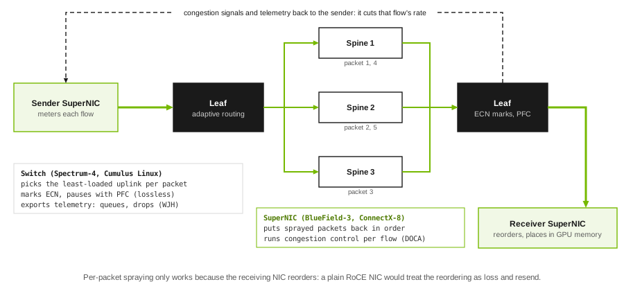
Few flows defeat hashing. ECMP picks a path per flow from a hash, and a training job has few, large, long-lived flows. With eight flows on eight uplinks, the chance that no two share an uplink is 8!/8⁸, about 0.24%. On average about 34% of the uplinks carry nothing while others carry two or more flows, and a collective runs at the speed of its slowest flow. RoCEv2 gets some entropy from the UDP source port per queue pair, and NCCL can open more queue pairs per connection (NCCL_IB_QPS_PER_CONNECTION), but hashing remains probabilistic. That’s the problem adaptive routing solves, on Quantum InfiniBand and on Spectrum-X, where NVIDIA describes the switch and SuperNIC working together to route RoCE dynamically.
Synchronized fan-in fills buffers in microseconds. When eight senders converge on one 400 Gb/s port, the excess is 2.8 Tb/s: the queue grows by 0.35 MB every microsecond. Shallow-buffered switches can’t absorb that for long, so the fabric has to slow senders (ECN, DCQCN) or pause them (PFC) before drops happen. With RoCE, a drop is expensive: many adapters recover by resending everything after the lost packet.
Oversubscription stretches every step. A 2:1 leaf is harmless when traffic is independent and spreads out. Collectives fill every uplink at the same moment, so a 2:1 ratio can double the exposed communication time, every step. The average utilization graph will still show the fabric half idle.
Failures reshuffle everything. When an uplink fails, plain modulo hashing moves most flows, not only the failed link’s, at the moment capacity just dropped. Resilient hashing, or adaptive routing, keeps the damage local.
Stragglers and jitter: the training-time penalty
A collective completes when its last participant completes. For a synchronous step:
T_step = T_compute + max over all ranks (T_exposed_comm,i)
The maximum is what makes AI fabrics unusual. If each of N ranks independently has a probability p of a hiccup in a given step (a retransmission, a congested queue, a slow link, a throttled GPU), the probability that the step is delayed is:
P(step delayed) = 1 − (1 − p)^N
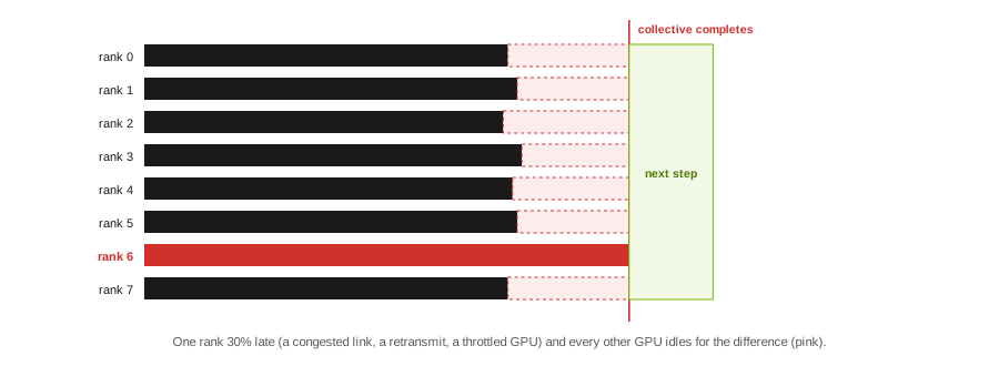
With p = 0.1% and N = 1,024 ranks, 64% of steps are delayed. Equivalently, the step time follows roughly the (1 − 1/N) quantile of the per-rank latency distribution: at 1,024 ranks you’re designing for the 99.9th percentile, not the median. Tail latency is the metric, and averages hide it.
A worked penalty. Take a 500 ms step, 1,024 GPUs, and that 0.1% chance per rank per step of a 10 ms delay. The expected delay is about 0.64 × 10 ms = 6.4 ms per step, 1.3% of the step. Over 30 days of training, that’s about 1.3% of 737,000 GPU-hours, or roughly 9,400 GPU-hours spent waiting, caused by events that would never register on a utilization graph:
T_train penalty ≈ steps × E[max delay] ≈ (1 − (1 − p)^N) × d × steps
This is why the troubleshooting domain spends so much time on single links and single counters. A port with a rising error rate on one rail can slow the entire job.
What NVIDIA’s reference designs do about it
NVIDIA’s reference architectures translate all of this into a handful of rules. The DGX SuperPOD reference architecture with H100 is the most detailed public example:
| Constraint from the traffic | Design rule | In NVIDIA’s reference architecture |
|---|---|---|
| Collectives fill every link at once | 1:1, full bisection bandwidth on the compute fabric | H100: a rail-optimized, balanced full fat-tree; GB200: a fully non-blocking fat tree per scalable unit |
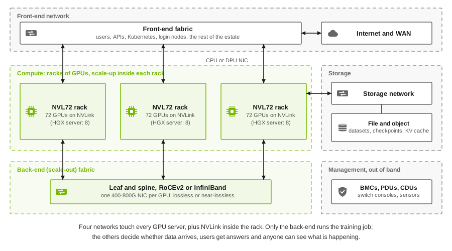
| Each GPU needs its own path out | One NIC per GPU, each on its own rail | Eight single-port ConnectX-7 cards at 400 Gb/s per DGX H100, one per GPU |
| Most traffic is between same-index GPUs | Rail-optimized leaves | Each group of 32 nodes is rail-aligned: one hop between same-rail GPUs in a scalable unit |
| Growth without redesign | Scalable units | 32 DGX per SU, 8 leaf and 4 spine switches per SU in the InfiniBand design |
| Storage bursts must not share queues with collectives | Separate fabrics | Separate storage, in-band management and out-of-band management networks |
| Chatty parallelism must stay off the fabric | Keep tensor parallelism in the NVLink domain | Eight GPUs per NVLink domain on DGX H100; 72 on NVL72 racks |
| Hashing can’t balance a few large flows | Adaptive routing and congestion control | Quantum InfiniBand adaptive routing; Spectrum-X switch plus SuperNIC adaptive routing and telemetry-based congestion control |
| Reductions double the bytes | In-network reduction where available | SHARP on Quantum InfiniBand; NVLink SHARP inside the NVLink domain |
Two practical notes. First, the exam’s Spectrum domain is about Spectrum-X running Cumulus Linux with NVUE, and the troubleshooting domain names Cumulus tools such as cl-resource-query; Onyx isn’t in the blueprint, so I’ll use Cumulus, DOCA and Linux tools throughout. Second, the blueprint lists NVIDIA’s DSX Air simulation, which is where most of the hands-on work in this series will run.
Checking a host and a job
Before blaming the fabric, check what the job actually sees. Illustrative commands; flags and outputs vary by release:
nvidia-smi topo -m                 # GPU-to-GPU and GPU-to-NIC paths: NV# (NVLink), PIX, PXB, PHB, SYS
ibdev2netdev                       # which RDMA device maps to which interface (DOCA host / MLNX OFED)
show_gids                          # RoCE GID table: the RoCEv2 GID index NCCL should use
ib_write_bw -d mlx5_0 --report_gbits <server>      # perftest: one NIC pair, no NCCL in the way

NCCL_DEBUG=INFO NCCL_DEBUG_SUBSYS=INIT,NET \
  mpirun -np 16 -H node1:8,node2:8 ./build/all_reduce_perf -b 8 -e 8G -f 2 -g 1
# INFO lines show the NICs, transports (IB / RoCE), GPUDirect RDMA use and the rings and trees chosen
NCCL_TOPO_DUMP_FILE=/tmp/topo.xml  # write the topology NCCL detected, to compare with what you expected
The NCCL settings that matter most for fabric design, from NVIDIA’s NCCL documentation:
| Variable | What it controls |
|---|---|
NCCL_IB_HCA |
Which RDMA devices NCCL uses; prefix with = for exact names |
NCCL_CROSS_NIC |
Whether a ring or tree may use different NICs on different nodes (0 keeps it on one rail) |
NCCL_PXN_DISABLE |
Turns off PXN, the NVLink detour to a GPU whose NIC is on the right rail |
NCCL_IB_QPS_PER_CONNECTION |
Queue pairs per connection, for more hashing entropy (1 to 128, default 1) |
NCCL_NET_GDR_LEVEL |
How close the NIC must be to the GPU for GPUDirect RDMA (LOC, PIX, PXB, PHB, SYS) |
NCCL_ALGO, NCCL_PROTO |
Force algorithms and protocols; for testing, not production |
On the switch side, a Spectrum-X switch running Cumulus Linux shows its RoCE configuration and counters with nv show qos roce and the interface counters. Those belong to the Spectrum articles; here the point is the order of work: confirm the job’s topology and baseline first, then go to the fabric.
Self-check
1. A 25 MB all-reduce over 1,024 GPUs is slow, while a 2 GB all-reduce on the same fabric reaches close to line rate. What dominates the small one, and what does NCCL do about it?
Latency. A flat ring pays 2(N − 1) per-step latencies, which at 1,024 GPUs dwarfs the 1 ms of data movement. NCCL uses double binary trees (logarithmic latency) and hierarchical algorithms, and in-network reduction where available.
2. nccl-tests reports an all-reduce algbw of 26 GB/s across 16 GPUs. What is the busbw, and what do you compare it with?
busbw = 26 × 2(15)/16 = 48.75 GB/s. Compare it with the per-GPU network rate: 50 GB/s for a 400 Gb/s NIC. That’s close to line rate.
3. Which parallelism should stay inside the NVLink domain, and why?
Tensor parallelism: it all-reduces inside every layer, two all-reduces in forward and two in backward per transformer layer, so it needs the highest bandwidth and lowest latency available.
4. Why can a 2:1 oversubscribed leaf double step time when its average utilization is under 50%?
Collectives make every GPU send at the same moment. Average utilization blends idle compute phases with communication bursts at line rate; during the burst, the uplinks carry half the demand, so the exposed communication takes about twice as long.
5. 512 ranks each have a 0.2% chance per step of a 5 ms stall. What fraction of steps is delayed?
1 − 0.998^512 ≈ 1 − e^(−1.02) ≈ 64%. Small per-rank risks become the common case at scale.
What’s next
Article 2 stays in the design domain: rail-optimized topologies and GPU-to-GPU paths, with the scalable-unit arithmetic, PXN and the cabling rules that follow from it. Then the series moves to the 60% of the exam that is Spectrum-X and InfiniBand.
References
- NVIDIA, NVIDIA-Certified Professional: AI Networking: exam details and blueprint weights, checked October 2026.
- NVIDIA, nccl-tests performance notes: algbw, busbw and the per-operation factors.
- NVIDIA, NCCL environment variables: NCCL_ALGO values (Ring, Tree, CollnetDirect, CollnetChain, NVLS, NVLSTree, PAT), PXN, CollNet, GDR level, IB settings.
- NVIDIA Technical Blog, Massively scale your deep learning training with NCCL 2.4: double binary trees.
- NVIDIA Technical Blog, Doubling all2all performance with NCCL 2.12: PXN.
- NVIDIA, DGX SuperPOD reference architecture (H100): network fabrics and key components: rail alignment, scalable units, separate fabrics. And the GB200 reference architecture: network fabrics: a fully non-blocking fat tree per scalable unit.
- NVIDIA, Spectrum-X: adaptive routing between switch and SuperNIC, telemetry-based congestion control.
- PyTorch, DistributedDataParallel: gradient buckets, 25 MB by default.
- Rajbhandari et al., ZeRO: Memory Optimizations Toward Training Trillion Parameter Models: communication volume 3Ψ for stage 3 against 2Ψ for data parallelism.
- Shoeybi et al., Megatron-LM, and Narayanan et al., Efficient Large-Scale Language Model Training on GPU Clusters Using Megatron-LM: tensor and pipeline parallelism and their communication.
- Related on this site: the six places an AI fabric congests, what ECMP hashing really does, oversubscription in AI fabrics and scale-up versus scale-out.
This guide follows NVIDIA’s public blueprint and documentation; it contains no exam content. Commands are illustrative: validate them against the documentation for your release. NVIDIA, NCCL, Spectrum-X, Quantum, BlueField and DGX are trademarks of NVIDIA Corporation.